Dartmouth BASIC: A Short Program Can Still Have State

A calculation can be easy to describe and tiresome to repeat. Square a number, add it to a total, move to the next number and do the same thing again.

The computer is willing to repeat the work. The programmer has to say what changes between repetitions, what stays, and when to stop.

Dartmouth BASIC gave beginners a compact language for that conversation. Its short statements made the machinery approachable, while leaving the important programming ideas intact. A loop still needs a counter. A total still needs somewhere to remember the terms already included.

That is the part worth looking at closely: a small program can have a surprisingly precise agreement with its own changing state.

Dartmouth, May 1964

Dartmouth’s institutional history dates the successful initial runs to May 1, 1964, and credits John Kemeny, Thomas Kurtz and undergraduate contributors. The project combined a language with shared access to a GE-225 computer.¹

The May 1964 first manual calls for ease of learning and fast compilation. An interactive language isn’t automatically an interpreted language. Numbered instructions, LET, PRINT and FOR/NEXT appear in that original guide.²

This article stays with that early vocabulary. Later home-computer BASIC dialects supplied their own syntax, facilities and habits. A modern example that merely looks nostalgic can easily belong to a different language version.

Our program is newly written using inspected early forms. Its companion check runs a modern model of the arithmetic and control flow, not the original Dartmouth compiler or terminal service.

Five squares, one total

Choose the sum of the squares of the integers from one through five. The expected terms are one, four, nine, sixteen and twenty-five. Adding them gives fifty-five.

A period-style program for this original example is:

10 LET S = 0
20 FOR N = 1 TO 5
30 LET S = S + N*N
40 NEXT N
50 PRINT S
60 END

The multiplication is deliberate. We don’t need to substitute a modern exponentiation glyph or assume that every mathematical convention of a later BASIC is present.

S holds the accumulated sum. N identifies the current term. The FOR and NEXT statements describe the repeated region, which contains the calculation at line thirty.

The source has six numbered statements. Its execution involves more than six statement visits because the loop returns to its body for subsequent values of N.

A short listing isn’t evidence that the machine does each line only once.

Assignment reads the previous value

The statement LET S = S + N*N can look odd if read as an algebraic equation. In ordinary algebra, subtracting S from both sides would say that N squared must be zero.

Here it is an assignment. Read the old S and current N, calculate the expression on the right, then store the result as the new S.

At the start S is zero. With N equal to one, the expression produces zero plus one: new S is one. With N equal to two, it produces one plus four: new S is five.

The variable name is the same on both sides, but the values belong to different moments. Confusing them makes a straightforward update look like an impossible equation.

Our checker explicitly records the before value, term and after value for each iteration. The first two records are (0, 1, 1) and (1, 4, 5). The old total is consumed once to produce the next total.

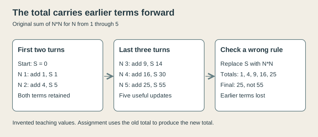Original explanatory SVG, created in 2026. Chosen values and a deliberately incorrect replacement rule; not a historical compiler display.

The final three totals are fourteen, thirty and fifty-five. Each incorporates everything that came before it.

The loop has a boundary

Starting N at one and ending at five gives five terms, including the upper bound. The original manual’s FOR/NEXT example describes that inclusive positive progression.²

Our teaching model checks N values [1, 2, 3, 4, 5]. The final added term is twenty-five, so a result of thirty would reveal that the fifth iteration was omitted.

Changing the upper bound to four intentionally produces thirty. Changing it to six produces ninety-one. These are useful nearby checks because they expose a wrong boundary that might be concealed by merely verifying a plausible-looking positive answer.

The example doesn’t depend on what value the historical implementation left in N after loop termination. The reported result is S, and the checker records the values used while the body actually runs.

That restraint matters when presenting period code. A modern loop model can confirm the intended five updates without proving every incidental detail of the original compiler’s final variable state.

Numbered source isn’t a stopwatch

The numbers ten, twenty and thirty identify source statements. They aren’t time intervals or promises about how long each instruction runs.

Within our example, source order places initialization before the loop and output after it. Loop control revisits the body rather than advancing monotonically through the labels on every execution turn.

The beginning of the conceptual trace is ten, twenty, thirty, forty, thirty, forty. Repeating thirty and forty is how the source describes repeated arithmetic without five copies of the calculation.

Leave gaps between labels and a new statement can be placed between existing ones. Insert 35 PRINT S between the update and NEXT. The existing labels can stay.

That makes the program print each intermediate total as well as the final total at fifty. It changes the observable behavior without changing the sum.

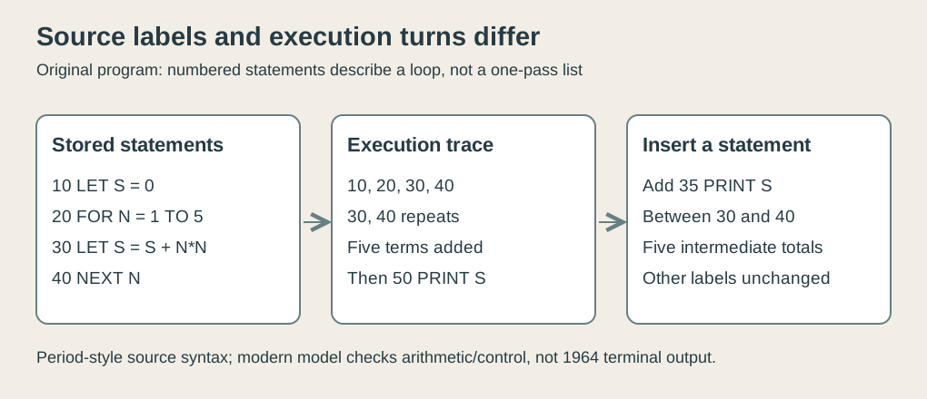Original explanatory SVG, created in 2026. Period-style source and a conceptual execution trace, not a reproduced terminal transcript.

The original manual recommends gaps for insertion.² Our chosen insertion makes that small editorial convenience concrete: a diagnostic observation can sit beside the update whose behavior we want to inspect.

Printing doesn’t repair the calculation

Intermediate output is useful because it reveals the progress of a value. It doesn’t itself make the rule correct.

Replace line thirty conceptually with LET S = N*N. The output sequence becomes one, four, nine, sixteen, twenty-five. Each value is a correct square, yet the final answer is twenty-five rather than fifty-five.

The loop visited the intended numbers. Multiplication worked. The error is that assignment replaced the total with the current term, discarding earlier terms.

A second incorrect model adds each term twice. Its totals become two, ten, twenty-eight, sixty and one hundred ten. Repeated output exposes that error too, but it takes an expected relationship to identify it: each increment should equal N squared once.

Our checker tests the good trace against that invariant and verifies the two deliberately wrong final answers. It doesn’t congratulate an incorrect program merely because it printed five numbers.

Initialization is part of the algorithm

The first line matters even though it contributes no square. It establishes the starting meaning of S: no terms have been included yet.

Begin S at one hundred and follow the correct loop. The final result is one hundred fifty-five. All five updates can be individually right while the overall answer retains an unintended starting offset.

For a chosen rerun model, initialize S again before each run. Two runs then both produce fifty-five. Deliberately retaining the previous final S produces one hundred ten on the second pass.

This is a model of an initialization mistake, not a statement that the Dartmouth service preserved variables in exactly that manner between RUN commands. The important obligation is local to the algorithm: the total must begin with the value the method assumes.

It is worth testing because initialization often looks like housekeeping. Here it supplies the base case on which every later update relies.

A relationship that predicts the next turn

After the kth completed iteration, S should equal the sum of the first k squares. At k zero, S is zero. If the relationship holds after k turns, adding the next square extends it correctly to k plus one.

That is a loop invariant: a statement about the state that remains true as repeated work advances. The phrase sounds more formal than the six-line program, but the idea is already present in its design.

The checker compares every accumulated value with a separately calculated sum, then checks final totals for bounds one through twenty. This goes beyond matching fifty-five once. It verifies that the same update method works across a small range of lengths.

The test environment uses modern Python integers. It doesn’t establish the limits or rounding behavior of the 1964 machine’s numeric representation, or recreate compilation, terminal editing and formatted output.

There is also a useful separation between the requested calculation and its presentation. Printing the final total once or printing every intermediate total changes what the reader sees. With the same initialization and updates, the mathematical result remains fifty-five. That lets observation support debugging without becoming part of the accumulation rule.

Small enough to inspect

I like this example because every useful piece has a visible responsibility. N chooses the term. S preserves previous work. LET changes state. FOR/NEXT revisits the calculation. PRINT makes a result observable.

The language can be approachable without pretending that programming is merely typing a formula. Its compact form makes it easier to see how a formula becomes a repeated procedure with a beginning, a changing state and an end.

The computer will patiently repeat the statement. The programmer’s contribution is deciding what that repetition is supposed to remember.

Footnotes

1. Dartmouth College, “BASIC Begins at Dartmouth”, institutional anniversary history. Used for May 1, 1964, GE-225 and collaborative origin, without adopting its sweeping first-system claims. ↩

2. First Dartmouth BASIC instruction manual, May 1964 first draft, preface and printed pages 4, 7, 9–10. Original scan inspected for compilation goal, numbered statements, assignment and inclusive positive FOR/NEXT. Worked program and numerical traces are original. ↩ ↩² ↩³