LISP: The Shape of an Expression

Replace BLUE with GOLD in a collection of symbols. That’s easy if the collection is flat. It becomes more interesting when one entry contains another collection, and that collection might contain another.

You want to preserve the arrangement while changing the selected symbols. Treating the whole thing as a character string gives you places to search, but leaves you to interpret what the parentheses and words are doing.

A structural representation gives the program something more useful: parts it can recognize, inspect and rebuild. The same rule can work through an expression at several depths.

Early LISP joined that representation to recursive functions. Its compact building blocks offered a way to handle symbolic relationships without inventing a separate storage layout for every shape of expression.

The parentheses are visible. The structure they describe does the work.

A beginning, rather than one launch day

John McCarthy’s creator history places the start of LISP implementation in fall 1958 at MIT’s Artificial Intelligence Project, which he and Marvin Minsky began. Early work used hand-compiled functions and supporting routines; Steve Russell later hand-coded an interpreter from the evaluation function.¹

The historical account is a retrospective, with McCarthy acknowledging gaps in its contributor coverage. The date therefore marks implementation’s beginning, rather than a complete modern language suddenly arriving in one release.¹

For the technical boundary, this article uses his April 1960 paper. It defines symbolic expressions from atoms and pairs, with operations for examining and constructing them. Its representation permits shared substructure but excludes cycles.²

That is enough for the original examples here. They don’t rely on Common Lisp, Scheme or a later dialect’s treatment of empty-list operations. A 1958 beginning isn’t permission to import every facility that later acquired the LISP name.

One list is a chain of pairs

Choose the invented list:

(RED BLUE GREEN)

In our teaching representation, a pair has two parts. The first refers to one element; the second refers to the rest of the list. The last pair’s second part is NIL, the terminating atom.

Give the three pair cells convenient labels R, B and G:

R = pair(RED, B)
B = pair(BLUE, G)
G = pair(GREEN, NIL)

Those labels are conceptual references, not historical addresses. Start at R and follow the second part to reach B, then G, then NIL. Follow each first part to obtain RED, BLUE and GREEN.

The paper’s car and cdr name the first and second parts of a non-atomic expression; cons constructs a pair. Under its definitions, taking car or cdr of an atom is undefined.² Our checker enforces that boundary instead of adopting a later runtime’s convenience rules.

The distinction between the first part and the rest is particularly useful. A traversal can take the current element, then apply the same procedure to the remaining chain. It doesn’t need a separate instruction for the fifth or fiftieth entry.

NIL supplies a stopping case. It doesn’t mean there must be another hidden cell containing a final empty item. It says that the chain has ended.

Add a head without copying the tail

Now put ORANGE before the existing three colors. Construct one new pair O whose first part refers to ORANGE and whose second part refers to R.

The new list reads:

(ORANGE RED BLUE GREEN)

The old root still points to R, so the old list still reads RED, BLUE, GREEN. Both roots reach the same three old cells.

The new structure contains one added pair rather than a newly copied four-pair chain. Sharing is possible because our model treats the existing pairs as unchanged objects. The new pair refers to the old tail; it doesn’t alter the old tail.

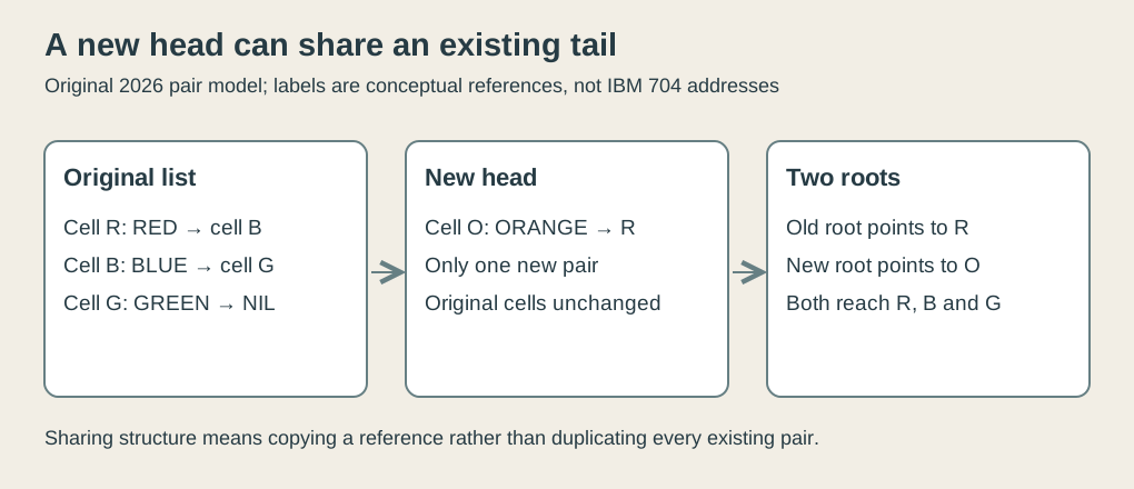Original explanatory SVG, created in 2026. Cell labels represent the invented immutable pair model, not IBM 704 storage addresses.

This provides a useful answer to “did the old list change?” The result’s printed notation contains another item, but the original root has not been redirected. Inspecting the original still yields the same sequence.

Identity and appearance are separate concerns. Two separately allocated chains can print identically without being the same cells. Our two lists print differently while sharing most of their structure.

The checker tests both relationships: the old list retains its contents, and the new head’s second part is the very same old root. A contents-only test would miss the sharing property.

If the pairs were freely mutated later, changing a shared cell could affect several roots. Our examples deliberately use immutable pairs, so that hazard doesn’t arise. This is a chosen teaching policy, not a claim that every historical or later LISP operation is purely functional.

A list can contain a list

The substitution problem needs a more interesting expression:

(RED (BLUE GREEN) BLUE)

Its outer list has three entries. The second entry is itself a two-entry list. The final BLUE is an ordinary outer entry; it isn’t inside the nested group.

Representing this with pairs takes five pair cells: three for the outer chain and two for the inner chain. The outer second cell’s first part refers to the inner list’s root. The links therefore describe both sequence and nesting.

A flat scan of the outer entries can find RED, the nested expression and BLUE. It won’t automatically find the inner BLUE, because that symbol is one level down. The substitution rule needs to inspect the contents of a pair, including nested parts.

Here is original explanatory pseudocode, using the same mathematical pattern as structural substitution:

replace(expression):
    if expression is an atom:
        if expression is BLUE: return GOLD
        otherwise: return expression
    otherwise:
        return pair(replace(first part), replace(second part))

The program recognizes two cases: an atom it can decide directly, or a pair whose parts require more work. Each recursive call receives a smaller piece of this finite expression.

BLUE becomes GOLD. RED stays RED. GREEN stays GREEN. NIL also remains NIL, so list endings are preserved.

The output is:

(RED (GOLD GREEN) GOLD)

Both appearances of BLUE changed, and the grouping survived.

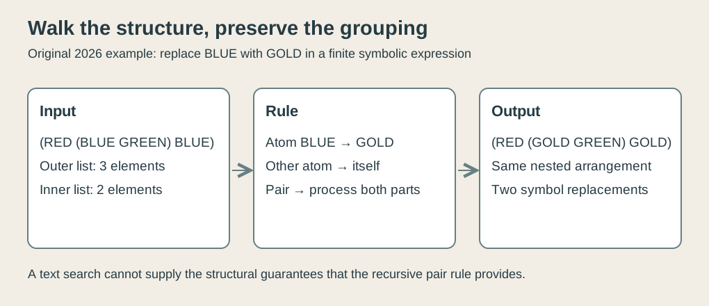Original explanatory SVG, created in 2026. The invented color symbols make two replacements and preserved nesting visible; this isn’t historical source or a terminal image.

The order of the cases matters

The atom test belongs before attempts to inspect a pair’s parts. Try to obtain the first part of BLUE itself and you’ve applied the pair operation outside its defined domain.

A structural program works because it respects the categories its representation supplies. It doesn’t succeed merely by making many recursive calls.

It also needs a terminating argument. In this finite model, a pair’s parts lead eventually to atoms. For the chosen nested list, the traversal visits five pair occurrences and six atom occurrences, including two NIL terminators. There are eleven calls in total.

That count is a useful check on the definition. Four visible color symbols appear in the printed input, but list structure contains terminating atoms as well. A test that only counts displayed words isn’t inspecting the complete representation.

A cycle would break this simple reasoning: following a link could revisit the same structure forever. The historical paper explicitly excludes circular structures; our original model likewise constructs only finite acyclic expressions.² It doesn’t silently borrow a later system’s circular-list behavior or invent a cycle detector for the original language.

Sharing remains different from a cycle. Two roots can refer to the same tail without that tail eventually pointing back to itself. The first saves duplication; the second changes the traversal’s termination problem.

Remembering unfinished work

While replacing the first part of a pair, the function must remember that its second part is still waiting. After obtaining both results, it constructs the replacement pair.

For the nested expression, this creates several outstanding pieces of work. The outer reconstruction waits while the inner list is processed. A recursive implementation needs a way to retain those partial results and return points.

Our modern checker uses Python’s call stack for that purpose. It doesn’t claim to reproduce an IBM 704 stack convention or the exact early LISP environment. The example establishes what information the procedure needs, regardless of how a machine stores it.

The naive reconstruction also creates five new pairs for our five old pair occurrences, even where a symbol stays unchanged. The original input remains available. A different teaching implementation could preserve some unchanged pair objects, but that would be another allocation policy to specify and test.

A result that prints correctly doesn’t by itself tell you how much storage was allocated. This is another reason to separate an expression’s logical contents from the graph of cells used to represent it.

An unused name isn’t unused storage

Return to the old list and its ORANGE extension. Stop retaining the original root R, while keeping the new root O. All four cells are still reachable: O leads to R, which leads through B and G.

The old variable’s disappearance doesn’t make its former tail disposable. Another live structure still needs it.

Reverse the situation: keep R but discard O. The original three cells remain reachable, while the extra ORANGE head no longer has a path from our retained root. This original reachability exercise explains why shared structures require more careful lifetime reasoning than “erase whatever the variable used to name.”

No historical garbage collector is being executed here. The checker simply counts reachable pair identities under two choices of roots. It verifies that the links actually justify the storage explanation.

Structure makes the rule reusable

I find the substitution example useful because its procedure stays small while the data’s arrangement can vary. It handles a flat list, a nested list or a pair-shaped expression by following the same two cases.

The representation supplies the categories. The recursive definition supplies the traversal. The chosen allocation policy preserves the original while producing a result.

LISP’s early symbolic approach made that combination expressible as a programming method. A collection of words became a structure that could be examined and transformed, and the program could reason through its parts without treating every new nesting depth as a new special case.

The parentheses are still there. Now they correspond to something the machine can work with.

Footnotes

1. John McCarthy, History of Lisp, retrospective draft dated February 12, 1979, especially “The implementation of LISP”. It distinguishes fall 1958 beginnings, hand compilation and Russell’s subsequent interpreter, while acknowledging incomplete contributor coverage. ↩ ↩²

2. John McCarthy, Recursive Functions of Symbolic Expressions and Their Computation by Machine, April 1960, symbolic functions and programming system. These are sections of one paper, supporting atoms/pairs, primitive domains, substitution and acyclic shared representation. All color lists, cell labels, pseudocode presentation and modern checks here are original teaching material. ↩ ↩² ↩³