System R and SEQUEL: Specify the Answer, Compare the Routes

A report needs approved invoices. The person asking probably cares which invoices appear, not whether the computer examines every record or follows an index to the useful ones.

That division of responsibility is attractive. It also gives the database a difficult job: choose an execution route that preserves the answer and uses reasonable resources.

System R investigated making relational requests practical. SEQUEL supplied a language direction in which users could describe wanted information through tables. The interesting engineering lies between the request and the chosen work.

Our original example will compare two routes, verify their answers independently and then give them an explicitly invented cost model. Cost is allowed to influence the route. It isn’t allowed to redefine the requested rows.

A research project with several phases

IBM’s publication record dates Donald Chamberlin and Raymond Boyce’s SEQUEL paper to May 1974.¹ The System R participants’ 1981 retrospective distinguishes Phase Zero in 1974–75 from the fuller multiuser construction in 1976–77 and experimental evaluation in 1978–79.²

Phase Zero supported a single-user subset with subqueries but no join construct, excluding concurrency and recovery. Later experimental installations weren’t a supported commercial product.²

Those boundaries prevent the opening year from inheriting every later capability. The relational model, SEQUEL, the initial prototype and a more complete implementation are related developments rather than one simultaneous product launch.

The detailed access-path paper discussed later in this article dates to 1979.³ Its optimizer should not be presented as already fully formed in the first 1974 prototype.

Define the answer before the cost

Invent an invoices table containing ten thousand rows. Each row has an integer identifier, an approval status and a chosen integer amount. For the first case, ten rows are approved.

Our requested answer is the set of identifiers for approved rows in one fixed table snapshot. We don’t request a particular output order, a sum or a limit on the number of rows.

That definition matters. If two implementations return the same set in different orders, they satisfy this request. If one misses an approved invoice, it is wrong even if it was wonderfully cheap to run.

The checker builds the ten thousand rows and derives the expected approved identifiers directly from their status. Then it implements scan and index routes separately and compares both with that expected set.

This is a modern Python data model. It doesn’t claim to execute original SEQUEL syntax, the System R storage subsystem or a 1974 join.

Route one: inspect every row

Our scan loops through the whole table, checks each status and retains the approved identifiers. It visits ten thousand rows and returns ten IDs in the first case.

For chosen cost accounting, imagine those rows occupying two hundred data pages. Charge two hundred page-work units plus one CPU-work unit for each inspected row.

To combine unlike kinds of work into one score, choose a CPU weight of 0.01. The scan’s score becomes two hundred plus one hundred: three hundred.

The score is neither elapsed seconds nor a count of actual reads performed by the Python checker. The page layout and weight are declared teaching assumptions.

A score can help compare plans only if the accounting convention is understood. Calling it milliseconds would add an unsupported precision that the model hasn’t earned.

Route two: use a selected index

Our index model maps each status to the identifiers of rows with that value. Looking up approved gives candidate IDs; the route then retrieves their records and rechecks approval before reporting the result.

Choose three page-work units for locating the index range and one further charged data fetch for each qualifying row. Charge one CPU-work unit for each such row, with the same 0.01 weight.

For ten matches, the index score is three plus ten plus 0.1: 13.1. Under these assumptions, the index route is much cheaper than three hundred.

Both routes still return the same ten identifiers. The optimization changes how we obtain the answer.

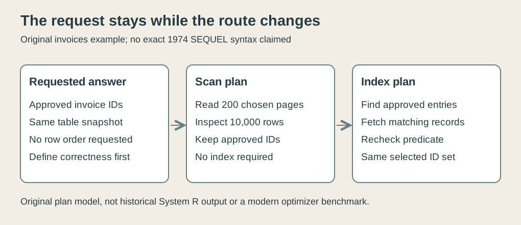Original explanatory SVG, created in 2026. Invented table and routes; no exact 1974 syntax, historical plan output or runtime benchmark.

The chosen per-record fetch charge describes a deliberately simple model without cache sharing. It doesn’t guarantee one distinct physical page for every record, or claim that a real implementation rereads a cached page each time.

More matches can change the decision

Keep the table size and scan score fixed. Now make one thousand rows approved. The index score becomes three plus one thousand plus ten: one thousand thirteen.

The scan still costs three hundred in our model, because it already examines every row. It becomes the preferred route.

An index exists in both cases. Its existence doesn’t establish that using it is always the better choice.

The fraction of rows that satisfy a condition is its selectivity. Our ten-match case selects one thousandth of the table; the thousand-match case selects one tenth. Those different quantities change the amount of work assigned to the index plan.

To locate the crossing precisely, write its score as three plus 1.01 times the qualifying count. At 294 matches the score is 299.94; at 295 it is 300.95.

Thus our discrete decision switches between those two counts. The checker uses exact decimal arithmetic for the scores, avoiding a rounding surprise near the boundary.

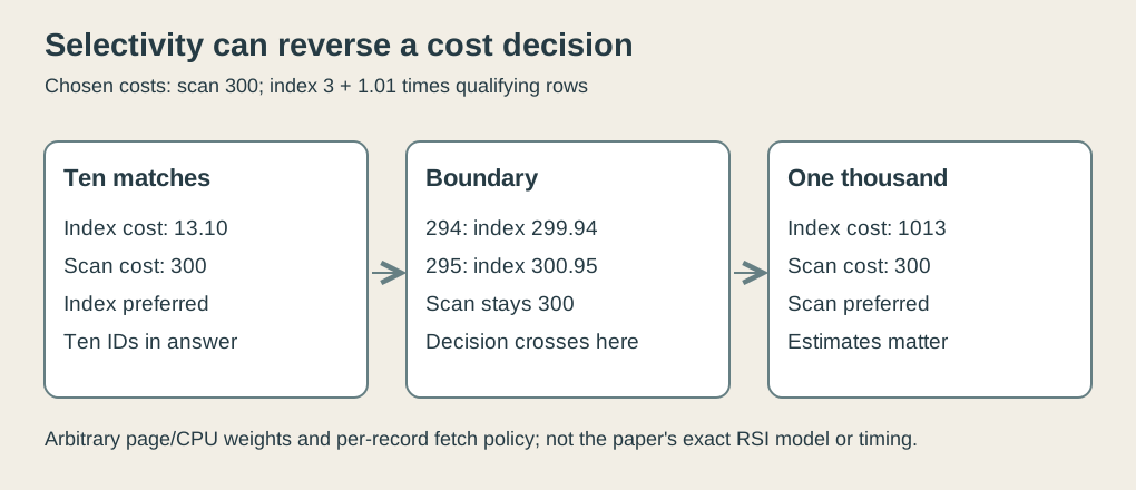Original explanatory SVG, created in 2026. Arbitrary weights and fetch accounting, not the historical paper’s exact RSI cost model or measured timings.

An estimate isn’t the eventual count

A planner has to choose before it has necessarily obtained the answer. Give our model an estimate of ten approved rows when the actual table contains one thousand.

The estimated score favors the index. Applying the same accounting to the actual count gives one thousand thirteen, while the scan would have scored three hundred.

The selected route remains correct: it returns the thousand approved IDs. The estimate made the performance choice worse, not the requested answer different.

That separation is useful when diagnosing a slow query. An inaccurate estimate doesn’t automatically mean a logically incorrect result. Conversely, a fast answer that omits rows isn’t successful optimization.

Our checker deliberately constructs this underestimate case and tests both properties independently: equivalent selected IDs and the wrong cost preference under stale input.

Change the weight, state the reason

CPU weight is another assumption. Suppose the weight becomes zero, so our score counts only chosen page work. The scan costs two hundred and the index costs three plus the matching count.

With weight 0.1, the scan costs one thousand two hundred; the index costs three plus 1.1 times the matching count. The boundary changes again.

Neither weight is inherently more truthful for every machine. The model needs a convention appropriate to what it is trying to compare.

The 1979 paper combines predicted page fetches with a weighted RSI-call term and uses catalog statistics for estimates.³ Our per-inspected-row CPU units are explicitly different from its exact storage-interface call accounting.

This distinction keeps the example useful without pretending that a simplified cost formula is a transcription of the historical implementation.

Layout can affect the fetch charge

Our index model assigns one fetch charge per qualifying row. A different layout assumption could put several matching rows together and reduce the number of data pages needed.

For an original alternative, suppose fifty qualifying records fit on each visited page and are packed consecutively. One thousand matches then need twenty data-page charges. With the three index units and ten CPU units, the score becomes thirty-three.

Under that chosen packed layout, the index beats the scan even for the thousand-match case. The logical answer is unchanged; a physical assumption changed.

The checker verifies this alternative separately. It doesn’t quietly replace the earlier accounting and then declare the original comparison wrong. Both results follow from their stated models.

A planner therefore needs information about more than the existence of an index. Counts, distribution and the way records are located can affect the work.

Empty answers still require work

Let no row be approved. Our scan still checks the table and costs three hundred. The chosen index route returns no IDs after its three-unit range lookup.

A zero-row answer doesn’t imply zero work. The route had to establish that no qualifying entries existed under the fixed snapshot and model assumptions.

Now let every row be approved. Both routes return ten thousand IDs, and our original per-record index score becomes ten thousand one hundred three. The scan stays at three hundred.

The checker covers both extremes as well as the crossing counts. They make it harder to accidentally confuse rows returned with rows examined, or to choose a route using a single ordinary example as universal evidence.

Give the optimizer room without surrendering the answer

I find this division of responsibility valuable because its boundaries are testable. The request fixes which data qualifies. Candidate plans offer different ways to obtain it. Estimates and costs help choose among those plans.

System R’s research explored making that arrangement work in a substantial database system. Our small examples show why the task involves both semantics and economics: correct alternatives can use very different amounts of chosen work.

The database can choose the route. The requested answer remains the agreement it has to keep.

Footnotes

1. IBM Research, SEQUEL publication record, May 1974, Chamberlin and Boyce. Abstract/metadata read; no exact original syntax asserted from it. ↩

2. Chamberlin and colleagues, “A History and Evaluation of System R”, 1981, pages 632–636. Project phases, initial subset and experimental status inspected. ↩ ↩²

3. Selinger, Astrahan, Chamberlin, Lorie and Price, “Access Path Selection in a Relational Database Management System”, 1979, pages 23–25, in a 2002 digital recreation. Actual paper read for cost/statistics context. All tables, scores and Python routes here are original models. ↩ ↩²